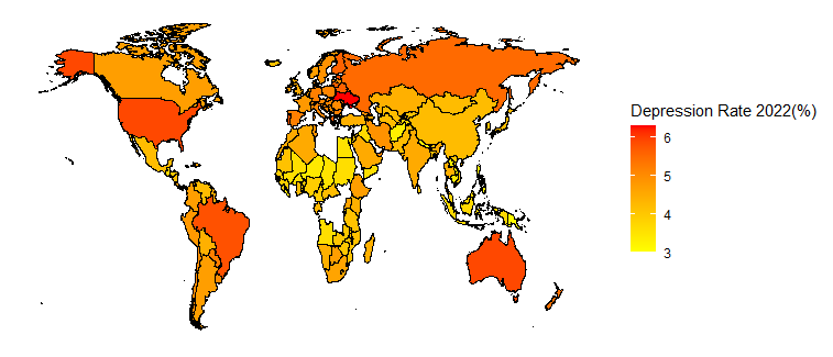
Depression is the disorder affecting the most people worldwide. Despite the great efforts made by the medical community, this complex mental health disease is still considered incurable^[1]. While there are a variety of effective treatments available for managing the symptoms of the illness, including medications, therapy, and lifestyle changes, there is no cure to the underlying disorder itself. Recent studies explored the trends in depression rates [Fig. 1], highlighting a concerning increase in the portion of the population affected by the disease in the last few years. There are ongoing debates among scientists about the potential drivers of this problematic growth. While the causes of depression are complex and varied, research has shown that both environmental and socio-economic factors can play a role in the development and severity of this illness. It is therefore of interest to analyse the statistical evidence surrounding the link between these factors and depression rates.

Our statistical analysis aims to investigate the correlation between socio-economical and environmental data of a country and its depression rate. We developed the same inquiry on a sample of countries worldwide and on the set of OECD countries. Ultimately, we tested whether OECD countries, considered by many as the most developed, display higher depression rates compared to other countries.

The Dataset

As previously mentioned, we developed our analysis on two separate parallel inquiries: the investigation of the drivers of depression on a sample of countries worldwide and on the set of OECD member states. The OECD, or the Organisation for Economic Cooperation and Development, is an intergovernmental organisation that works to promote economic growth, prosperity, and sustainable development in its member countries. It currently has 37 member countries, including some of the most developed ones. We built two different datasets for our study in order to individually focus on the two samples. There are multiple reasons why we chose to also analyse OECD countries on a stand alone basis. First of all, developed countries are arguably more inclined to provide unbiased, high-quality and up-to-date data. Secondly, the OECD is a sample of reasonable size from which to gather our data because its number of members is small but still sufficiently large to carry out a statistical study. In addition, the OECD publishes a great amount of open-source datasets on its website. Lastly, our global-scale inquiry lacks some of the data that is available for the most developed countries only.

In order to represent our dependent variable, i.e. depression, we used the latest available data regarding the percentage of population affected by the disease in several countries. Then, we proceeded building our datasets by looking for data relative to possible drivers of depression in a country’s population. These drivers can be divided into three main macro-categories: “social”, “economical” and “environmental”. The factors taken into account are the following:
-        Social: peacefulness, education level, internet usage.
-        Economical: income inequality, wealth
-        Environmental: weather, urbanisation

In the inquiry concerning OECD countries, we were able to additionally include working hours as an independent variable.
Peacefulness is indicated in both datasets by the 2022 GPI index, or Global Peace Index. We represented the education level in countries worldwide using the 2019 Education Index. For OECD countries, on the other hand, we fulfilled the same purpose by using data relative to the percentage of the countries’ populations which have not pursued upper secondary education^[2]. Average internet usage is represented in both inquiries by the percentage of a country’s population browsing the internet in 2017. Income inequality is described in the two datasets using the latest GINI indices (obtained by two different sources). We collected GDP per capita data for both inquiries in order to represent a population’s average wealth. We considered the countries’ average temperatures as a variable to evaluate the potential impact of weather. Urbanisation is captured by the percentage of the population living in urban areas. Lastly, average labour time was included in the OECD dataset to describe the amount of labour in each country’s population.

For each country, we merged the information relative to these indices to the corresponding depression rate. Then, we cleaned our data by filtering out those countries which lacked information on at least one of the variables taken into consideration. The final global and OECD datasets had sizes of 140 and 37 countries, respectively.
To compare the depression rates between members of the OECD and those which are not members, we had to build a third dataset, which contains all non-OECD countries in the global dataset.

Multivariate Linear Regression

Multivariate linear regression is a statistical method that allows us to understand the relationship between a multidimensional dependent variable and independent variables, also known as predictors or explanatory variables. The multiple linear regression model for n dependent variables Y1,...,Yn with corresponding p-dimensional predictor variables (X1,1,...,X1,p),...,(Xn,1,...,Xn,p) is described by the formula:

where e1,. . ., en are independent normally distributed random variables with expectation 0 and finite variance

In this section we are going to interpret the multivariate linear regression associated with the correlation between socio-economical and environmental data of a country and its depression rate: respectively our independent and dependent variables. We repeat this operation considering both the Global dataset and OECD dataset.

First off, we calculated the regression coefficients for each independent variable. These coefficients represent the strength and direction of the relationship between depression and the corresponding independent variables. Ideally, after calculating all regression coefficients, we could predict the depression rate of a country on the basis of the x values only. In computing our model, we conventionally took as our initial hypothesis that the coefficients’ value is 0, meaning that there is no relationship between the x variables and the y variable. Therefore, if our test yields low p-values, we witness significant correlations between the independent and dependent variables.

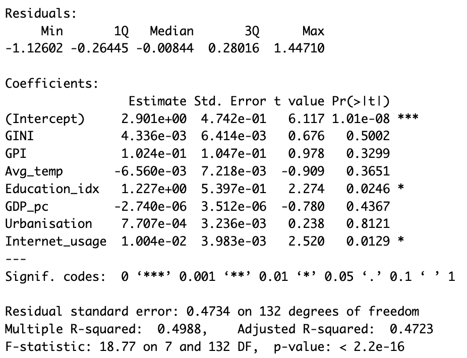
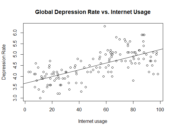
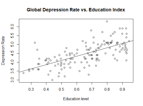
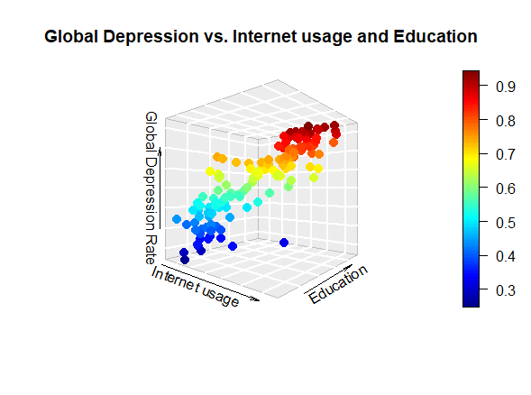
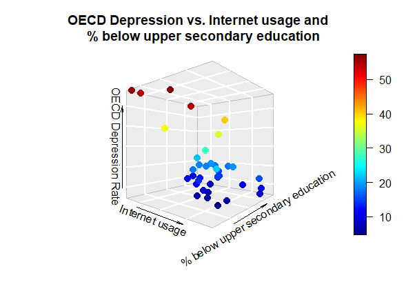
Interpreting the results relative to the Global dataset, we observe that the p-value of the F-statistics is p-value: < 2.2e-16, well below 0.05. This means that at least one of the predictor variables is significantly related to the dependent variable. By examining the coefficient table, which shows the estimate of regression beta coefficients and the associated p-values, we can gather that Education and Internet usage are statistically significant because their p-value is smaller than 0.05^[3]. Then, to understand if the correlation is positive, we keep in mind that a positive coefficient estimate suggests that an increase in the predictor variable produces an increase in the dependent variable. In our case, both Education and Internet usage [Fig. 2, 4, 6] are positively correlated to depression. The overall quality^[4] of the model can be assessed by examining the R-squared and Residual Standard Error, which represents the proportion of variance in the outcome variable y that may be predicted by knowing the value of all x variables. An R-squared value close to 1 reveals that the model is able to represent a large portion of the variance in the outcome variable. The Residual Standard Error estimate gives a measure of error of prediction. The lower the Residual Standard Error, the more accurate the model. In our model the Residual Standard Error is 0.4734 on 132 degrees of freedom. Therefore, we can deduce that our model is quite accurate^[5].
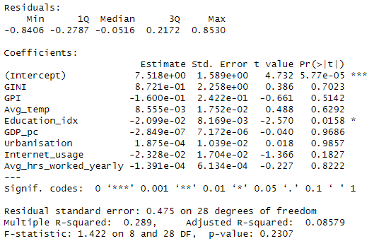
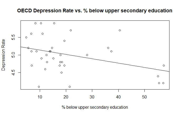
The results found using the OECD dataset are consistent with the outcomes depicted above. However, we observe that Education [Fig. 5] is the only statistically significant variable. In contrast with the Global inquiry, Education is negatively correlated to depression, for the reasons mentioned in section “The Dataset”. In the next section, using model selection methods, we will see how it is possible to find other statistically significant variables.

Overall, multivariate linear regression is a useful tool for understanding the relationships between variables and making predictions based on those relationships. However, by including all parameters we risk overfitting the model. As a result, the model may perform well on the training data, but not generalise to new data. In order to overcome this problem we will use model selection methods and check whether the assumptions required to state the statistical significance are met.

Model Selection

As previously stated, it is not always the optimal choice to include all measured predictor variables in the regression model. A way around this problem is to use model selection, a technique whose scope is to find the best-fitting model that is effective at making predictions or understanding relationships in the data. Model selection is important in statistical studies because it allows us to identify the most relevant variables and to avoid overfitting.

In this section we will exploit two different approaches to model selection, the Step-up and Step-down methods. Then, we will compare their output to the initial model using AIC.
The step-up method takes an empty model including the intercept only, and no parameters. Firstly, it tests all H0 :

separately and, if none of the hypotheses are rejected, we keep the empty model as our optimal. Otherwise, if any are rejected, we include in the model the parameter with the lowest p-value. Hence, we iterate the scheme enlarging our model until no parameters with p-value lower than our significance level are left.
The step-down model is specular to the step-up. We start off with the full model including all parameters and we test all H0 :

separately. If all of them are rejected we choose the full model; otherwise we remove the

with the highest p-value. We iterate the procedure keeping the smallest model, until all remaining parameters have p-values below the significance level.

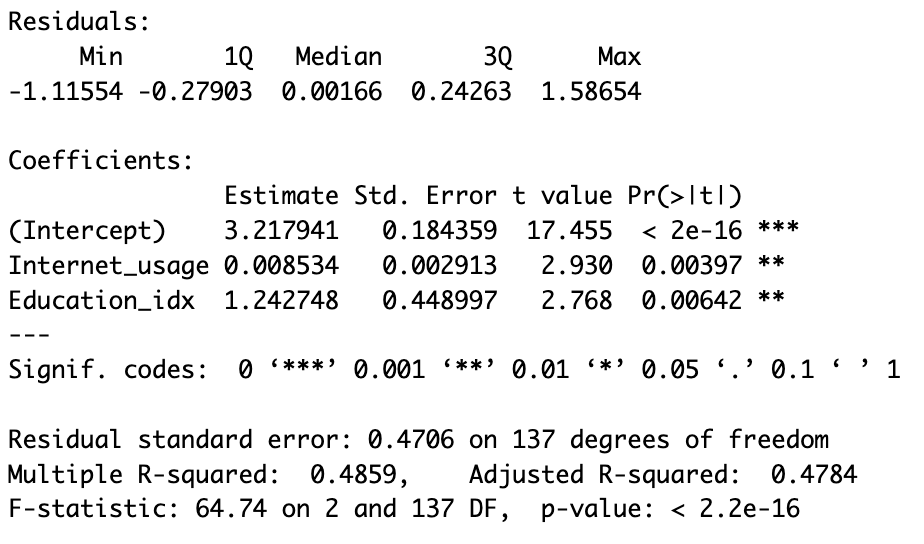
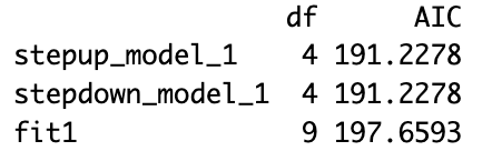
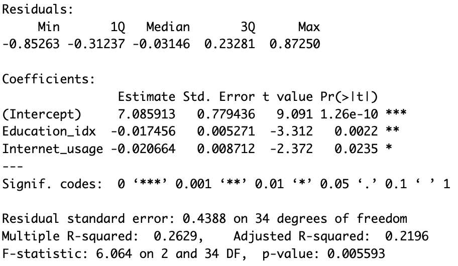
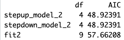
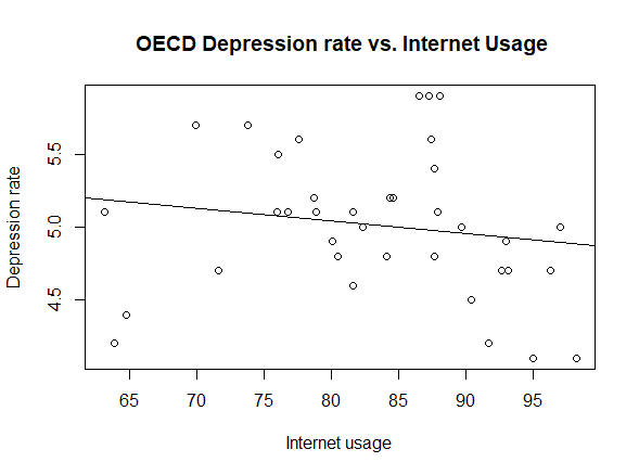
In both methods, we find that the optimal model is dependent on Education and Internet usage only^[6]. To check whether our selected models are statistically better than the one found via multivariate linear regression, we apply the Akaike’s Information Criterion. AIC is a statistical measure that is used to evaluate the quality of a statistical model. It takes into account both the goodness-of-fit of the model and its complexity, with the goal of finding the model that strikes the right balance between these two factors. AIC allows you to compare different statistical models and select the ones that are most likely to be the best fit for your data. This tool can only be used by reasonably assuming that we are dealing with sufficiently large datasets. Comparing the three models with AIC we get a higher coefficient for the full model and an equal coefficient for the step-up and step-down models. Thus, we deduce that the step-up and step-down models, containing the only two explanatory variables (i.e. Education and Internet usage) are qualitatively best. This result is consistent in both inquiries. However, we surprisingly observe that Internet usage is directly proportional to depression in the Global regression, whereas it is inversely proportional in the OECD inquiry [Fig. 3, 7]. We will later discuss possible reasons why this might have happened.

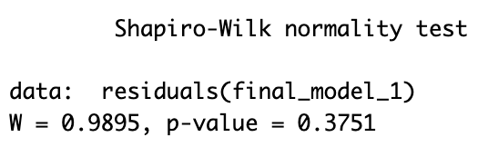
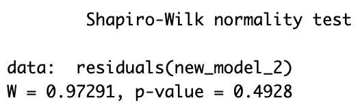
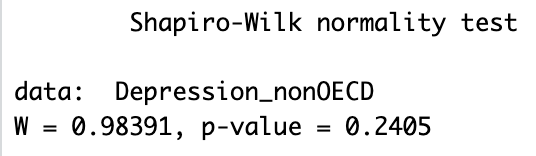
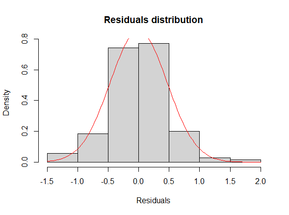
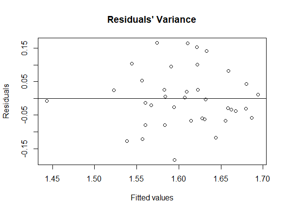
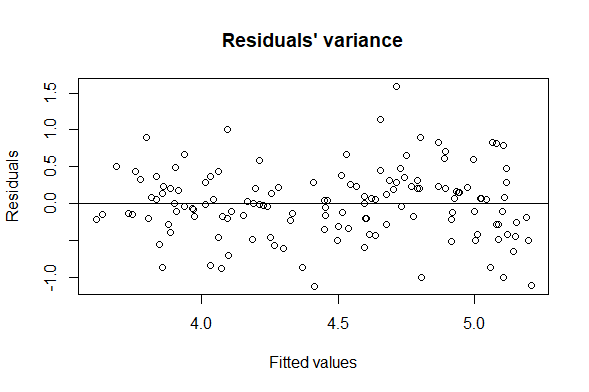
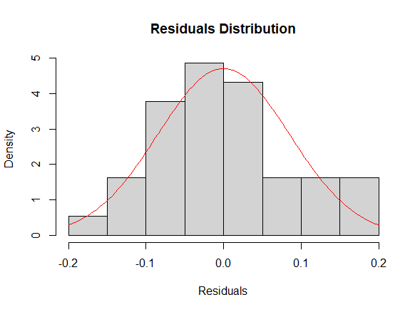
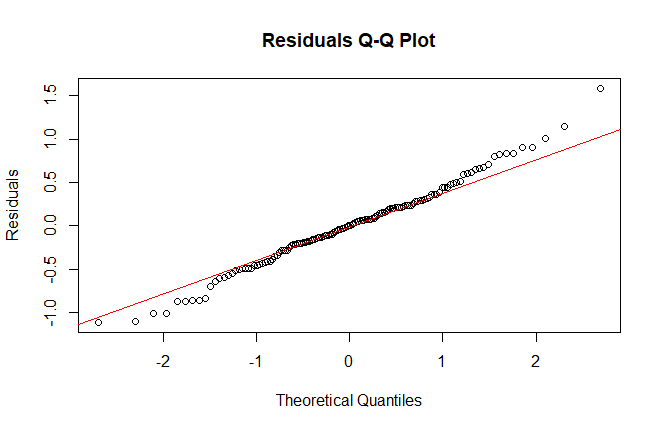
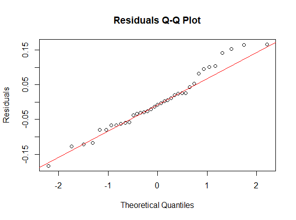
Lastly, we used the final model obtained with the step-up method to check the assumptions on the residuals, namely their normality, their homoscedasticity [Fig. 8, 9] and that their mean value is close to 0. In order to prove normality of the residuals, we visually observed their gaussian-shaped distribution with a histogram [Fig. 10, 11], verified the shape of their qq plot [Fig. 12, 13] and computed their corresponding Shapiro-Wilk tests. To check homoscedasticity, we graphically inspected whether the residuals’ variance was close to being constant. Computing their mean value, we are able to evaluate whether it is reasonably close to 0. All assumptions were satisfied, meaning that we could assess the results of the regression with the new model.

Hypothesis Testing

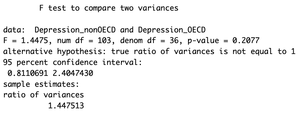
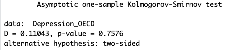
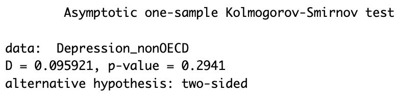
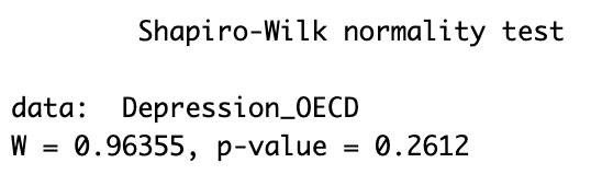
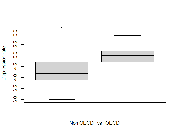
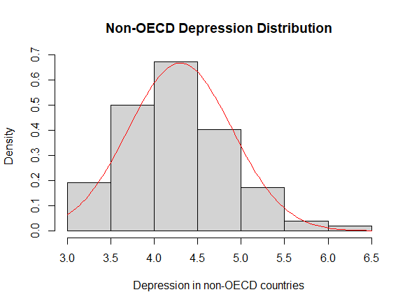
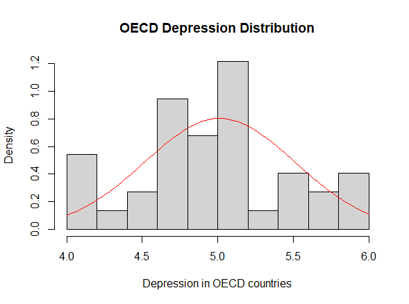
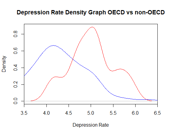
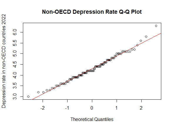
After comparing our analyses, it is of interest to learn whether OECD countries are significantly more depressed than non-OECD countries. In order to do so, it is reasonable to perform a student’s two-sample t-test. However, it is first essential to prove the prerequisites for t-testing: independence, homoscedasticity and normality of the dependent variables. Arguably, we can assume that depression rates in OECD countries are not correlated in any way to those in non-OECD countries (thus implying independence). Furthermore, to attest homoscedasticity in the two models, it is enough to perform a variance test or visually observe the resemblances of their corresponding boxplots [Fig. 14]. Lastly, to check normality, we can assess a series of dedicated tests, such as the Kolmogorov-Smirnov test and the Shapiro-Wilk test, and visual approaches, for example by plotting their histograms [Fig. 15, 16] and qq plots [Fig. 17, 18].

Our null hypothesis is

, where

is the mean of the depression rate in OECD countries and

is the mean of the depression rate in non-OECD countries. Specularly, the alternative hypothesis is

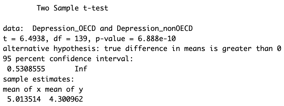
. Performing the test, we conclude that we must reject the null hypothesis. As a matter of fact, we observe that the test statistic belongs to the confidence interval, and the resulting p-value is much smaller than the significance level of 0.05. Thus, we establish that OECD countries have a significantly higher depression rate than non-OECD countries [Fig.19].

Conclusion

To sum up, we found statistical evidence of direct significant correlation between the depression rate and average education level of a population. Moreover, we surprisingly ran into opposite conclusions when assessing the link between depression and the internet usage in a country. While higher internet usage is a driver of depression in our global inquiry, in the OECD analysis we observe that internet usage influences our dependent variable in the other way around. Lastly, as a result of our hypothesis testing, we manage to draw the strong conclusion that OECD members witness an averagely higher depression than non-OECD countries.

The greatest limitation in our study is arguably represented by the choice of handling data regarding OECD countries. As a matter of fact, with all the advantages following our strategy, comes a great issue. OECD members are not a generic sample of countries in the world. On the contrary, they represent the most developed societies. This implies that, generally speaking, OECD countries share some very similar characteristics. For this reason, when choosing to analyse this dataset, we run the risk of producing a biased analysis. When studying the correlations to depression rate, we must keep in mind that this subset of countries share, for example, very similar internet usage percentages. Therefore, since this variable ranges in a very small interval [figure 3], it becomes hard to distinguish its link with depression. This condition is the possible reason why our analysis yielded two different, opposite, conclusions when assessing the link between internet usage and depression.
Another possible weakness of our analysis is the choice of the indices representing our independent variables. For example, temperature isn’t always linked to the typical weather of a country: it is not a direct implication of the amount of sunlight, fog, rain in a region. For instance, it could have been of interest to distinguish our countries by their climate region of belonging, rather than their temperature.

A fascinating future addition to our inquiry could be the focus on the effects of the recent COVID-19 pandemic on the depression rates of the involved nations. Moreover, if the relative data were available, it would be curious to repeat the same study by distinguishing the depression rates of female and male populations in a country.

Appendix

Saveanu, R.V. and Nemeroff, C.B., 2012. Etiology of depression: genetic and environmental factors. Psychiatric clinics, 35(1), pp.51-71.

Renaud-Charest, Olivier, et al. "Onset and frequency of depression in post-COVID-19 syndrome: A systematic review." Journal of psychiatric research 144 (2021): 129-137.

Goodwin, Renee D., et al. "Trends in US Depression Prevalence From 2015 to 2020: The Widening Treatment Gap." American Journal of Preventive Medicine 63.5 (2022): 726-733.

[2] Keep in mind that we used two indicators of education with opposite values in the two datasets (high education indices are reasonably comparable to low percentages of populations which have not pursued upper secondary education). We therefore expect that their correlations to depression, if any, are respectively opposite.

[3] Conventionally, in fact, we consider our significance level to be α = 0.05.

[5] To formally prove this, we can estimate the error rate by dividing the RSE by the mean outcome variable. In our case, the error rate is found to be 0.1055956 in the Global analysis, and 0.09473589 in the OECD analysis, which is fairly low.